I have fond memories of getting primary school pupils to explore the image filters in Photoshop substitutes such as GIMP and Pixlr, producing some Warhol-esque grids of portraits with different effects applied to each. Since them, image filters have become pretty much ubiquitous thanks to Instagram and the like, and so pupils’ familiarity with the idea can now be taken (almost) for granted, but I wonder how many of them pause and think about what’s happening behind the touchscreen?

I was quite taken with Mark Guzdial’s ‘MediaComp’ ideas as a way into programming for those who were inexplicably more interested in working with digital media than finding the sum of all the multiples of 3 or 5 less than 1000.

I’ve subsequently used image manipulation in whole cohort lectures to our BA Primary Education students, demonstrating how digital images are represented as red, green and blue colour values, and using GP as a block-based language to illustrate what happens when these values are changed.

You can do a similar thing in Excel, using Andrew Taylor’s rather brilliant JPEG -> Excel converter, as demosntrated by Matt Parker.

More recently, I’ve included similar exercices in Processing for our BA Digital Media students as part of their Software Studies module. There’s more of a learning curve here, but this is quite an accessible project once you’re used to Processing’s way of doing things.

Pillow Talk

In secondary schools, (almost) everyone is learning to code in Python, and almost everyone is learning how images are represented digitally as bitmap graphics. I think the former often gets taught through rather dull exercises which appear to involve doing things with integers and strings; the latter seems to involve colouring in on squared paper. I think there’s a quick win here: give pupils a real understanding of how actual images are actually represented using red, green and blue colour values, and have them coding in Python to do something that they wouldn’t have been able to do back in primary school using Scratch.

From what I’ve seen, the simplest way into image manipulation in Python is using the Pillow, the ‘friendly’ fork of the Python Image Libary (PIL). Rather than working in the (really quite unpleasant) IDLE, I’d recommend using a Jupyter Notebook for this, to encourage a dialogic style of programming: ask the interpreter to do something, then look at how it responds. Now ask it to do something else. You can install and run Jupyter on your own machine via the browser (or Nteract, or in VSCode), or just use the free, hosted Colab version of this from Google. If you’d like to follow though my examples, open my Notebook in another browser window.

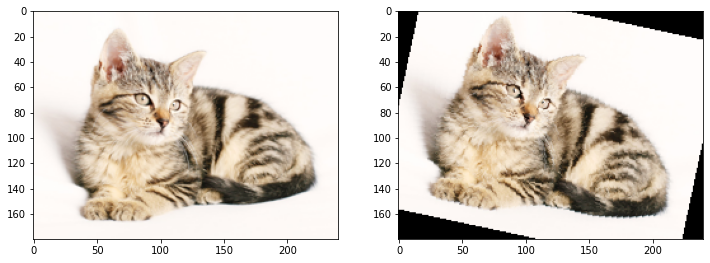
Pillow comes with some image manipulation methods built in - it’s easy enough to rotate an image:

rotated_image = image.rotate(-12)

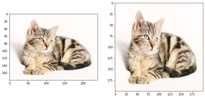
Or to resize and/or reshape the image, which would be useful for building a thumbnail gallery in a webapp.

resized_image = image.resize((200, 200))

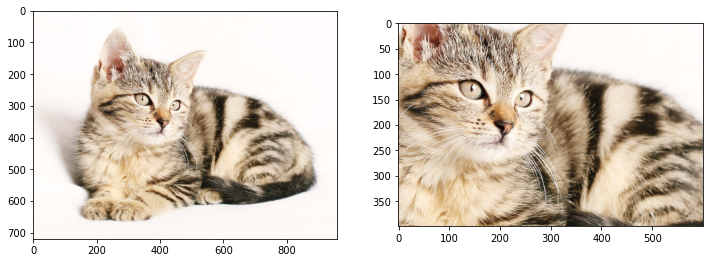
And to crop in on a particular part of the image:

cropped_image = image.crop(box = (200, 150, 800, 550))

Coding is the new Instagram

The fun starts though when you start playing with the getpixel and putpixel methods to start manipulating the red, green and blue values of each pixel.

In all of the examples here, the pattern is pretty much the same: iterate over each pixel, determine it’s current RGB value, change those according to some mathematical operation, and then set that as the new RGB pixel value.

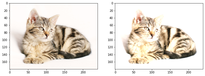
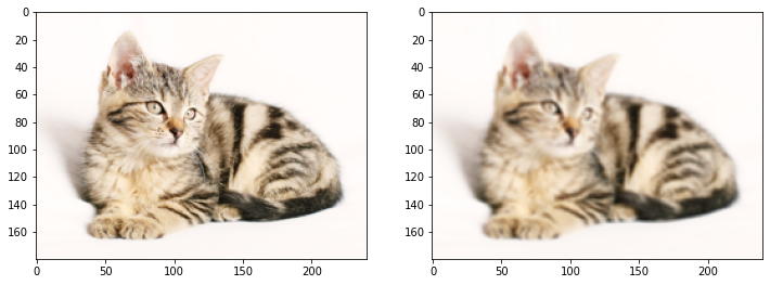
We might start by increasing the red, green and blue values of each pixel by the same amount, to make a brighter image:

brightness = 1.2
for x in range(width):
  for y in range(height):
    oldpixel = image.getpixel((x, y))
    newpixel = (int(min(oldpixel[0] * brightness, 255)),
              int(min(oldpixel[1] * brightness, 255)),
              int(min(oldpixel[2] * brightness, 255))) 
    image2.putpixel((x, y), newpixel)

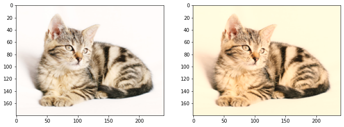
The colour balance can be changed - making a ‘warmer’ image involves increasing the red values whilst decreasing the blue:

for x in range(width):
  for y in range(height):
    oldpixel = image.getpixel((x, y))
    newpixel = (int(min(oldpixel[0] * 1.1, 255)),
              oldpixel[1],
              int(oldpixel[2] * 0.9)) 
    image2.putpixel((x, y), newpixel)

You’ll notice that in both of these examples, I’m doing a little extra maths to keep colour values constrained as whole numbers in the range 0 to 255. It might be more elegant to write a function to do that, but I’m inclined for an exercise like this to expose a bit more of the how the magic works. Abstraction has its place, but there are occasions when you want to show pupils what happens inside at least the first black box.

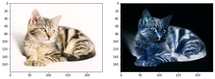
Some readers will be old enough to remember when photos were taken using chemicals on transparent plastic (no, really, I’m not making this up), and getting the origial, developed ‘negative’ as well as the printed photo. You can recreate this digitally by taking each of the colour values away from 255, although I’m not quite sure why you would want to.

for x in range(width):
  for y in range(height):
    oldpixel = image.getpixel((x, y))
    newpixel = (255 - oldpixel[0],
              255 - oldpixel[1],
              255 - oldpixel[2]) 
    image2.putpixel((x, y), newpixel)

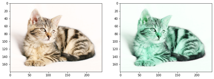
A similarly freaky effect can be achieved by swapping the data around between colour chanels. Here red becomes green, green becomes blue and blue becomes red. Again, I’m not sure that this will get you lots of likes on ‘stagram.

for x in range(width):
  for y in range(height):
    oldpixel = image.getpixel((x, y))
    newpixel = (oldpixel[2], oldpixel[0], oldpixel[1]) 
    image2.putpixel((x, y), newpixel)

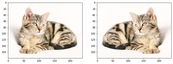
A mirror image involves taking the pixels from the right hand side of the rows and putting them at the left hand side of the new rows, and vice versa. Whatch out for the potential for an off-by-one error here. A left-right inversion still looks like a cat. A top-bottom one just looks like an upside down cat. You’ll have noticed that gravity works downwards. By definition.

for x in range(width):
  for y in range(height):
    newpixel = image.getpixel((width - x - 1, y))
    image2.putpixel((x, y), newpixel)

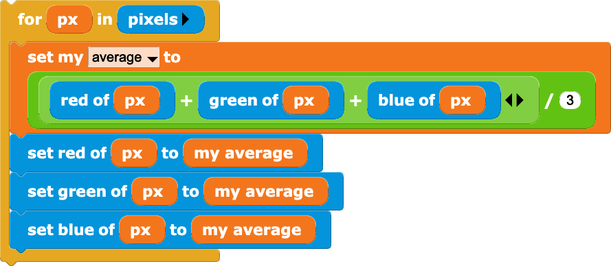
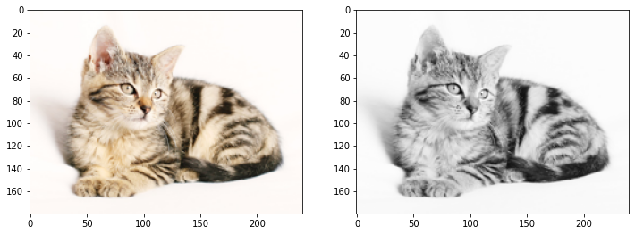
If the red, green and blue channels are all set to the same value, we get a grey-scale image. Here, I’m setting all three values to the mean of the red, green and blue values, but there are other ways to do this. I have a soft spot for moody black and white pictures…

for x in range(width):
  for y in range(height):
    average = sum(image.getpixel((x, y))) // 3
    image2.putpixel((x, y), (average, average, average))

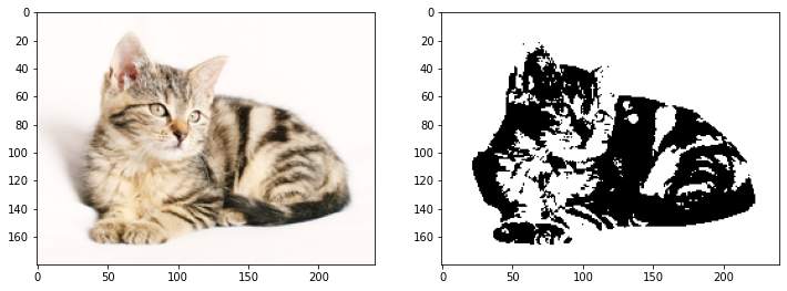
We’ve reduced the colour depth from c 16 million colours here (24 bits) to just 256 shades of grey (8 bits). We can reduce it further still, to just one bit per pixel:

threshold = 192
for x in range(width):
  for y in range(height):
    average = sum(image.getpixel((x, y))) // 3
    if average >= threshold:
      value = 255
    else:
      value = 0
    image2.putpixel((x, y), (value, value, value))

Increasing or decreasing the saturation is a bit more complicated, but essentially this is about increasing or decreasing the difference between each of the channels and the average grey scale values. Again, the code is made a bit more complicated by the need to constrain values to integers in the 0 to 255 range. The eagle eyed will spot that I’m iterating across a mutable list of colour values at each pixel, but then casting the list as a required tuple for setting the pixels of the new image.

saturation = 1.5
newpixel = [0, 0, 0]
for x in range(width):
  for y in range(height):
    oldpixel = image.getpixel((x, y))
    average = sum(oldpixel) // 3
    for i in range(3):
      newpixel[i] = int(
          max(
              min((oldpixel[i] - average) * saturation + average, 
                  255),
              0))
    image2.putpixel((x, y), tuple(newpixel))

One way of blurring the image is to replace the values of each pixel with the average of those in the box around them - in this case the 3x3 grid, but a bigger box gives a more blurry image.

for x in range(1, width - 1):
  for y in range(1, height - 1):
    newpixel=[0, 0, 0]
    for dx in range(-1, 2):
      for dy in range(-1, 2):
        nearby=image.getpixel((x + dx, y + dy))
        for j in range(3):
          newpixel[j] = newpixel[j] + nearby[j]
    newpixel = tuple([x // 9 for x in newpixel])
    image2.putpixel((x, y),newpixel)

It’s convoluted

Another way of doing this is through a convolution with a simple matrix. For each of the colour chanels, we multiply the values in the 3x3 box around our target pixel with the corresponding number in the ‘kernel’ matrix, adding together these products.

Whilst this is harder to explain (and moves us beyond Key Stage 3 maths, and possibly beyond what would normally be expected in Key Stage 3 computing), it’s a more flexible approach with wider applications, as we’ll see.

In code, we first define the kernel matrix:

kernel = [[1, 1, 1],
          [1, 1, 1],
          [1, 1, 1]]

and then we can write a function to scale the kernel down (forgive the list comprehension here) and do the convoluted product and sum:

def convolve(kernel,image):
  weight = sum([sum(row) for row in kernel])
  if weight != 0:
    kernel = [[cell / weight for cell in row] for row in kernel]

  image2 = Image.new("RGB", (image.width, image.height))
  
  for x in range(1, width - 1):
    for y in range(1, height - 1):
      newpixel = [0, 0, 0]
      for dx in range(-1, 2):
        for dy in range(-1, 2):
          nearby = image.getpixel((x + dx, y + dy))
          for j in range(3):
            newpixel[j] = newpixel[j] + 
            nearby[j] * kernel[1 + dy][1 + dx]
      newpixel=tuple(map(int, newpixel))
      image2.putpixel((x, y), newpixel)
  
  return(image2)

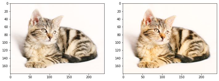
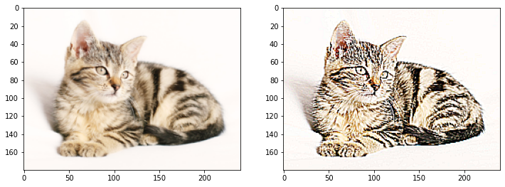
With the above kernel, we just get another blurry cat, as we’re still just taking an average of the nine pixels in the surrounding box, but this approach comes into its own when we change the kernel. For example, increasing the weighting of the middle pixel, whilst decreasing that of the ones around it, i.e. a kernel of

produces an impressive sharpening effect:

But then reducing the weighting of the middle pixel by just one, so that it balances the edge pixels exactly, gives us an edge detection convolution.

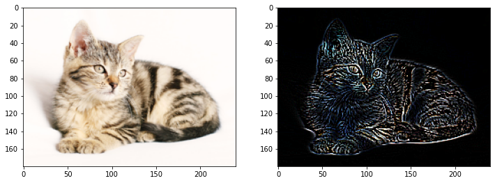
In the classroom, edge detection could be a nice example of the ‘hiding complexity’ approach to teaching abstraction, showing just the parts of the image where things change, so essentially the outline. It’s also important in computer vision machine learning based on convolution neural networks.

There’s an interactive version of the code for all the above in a Jupyter Notebook hosted on Google Colab. I’d encourage you to play around with the parameters, and do let me know if you try any of this out with your students.